As the Red Hat Summit shifts to the west coast in San Francisco this year Hortonworks and Red Hat will be demonstrating the progress of our engineering efforts. Our engineers have been hard at work in the factories and in the communities deeply integrating our open source offerings to create a comprehensive platform for new analytic applications. As a reminder in February Red Hat and Hortonworks announced a comprehensive open source initiative to deliver infrastructure solutions to bring 100-percent open source Hadoop to the hybrid cloud.
New to this initiative is integration of HDP with OpenShift. With OpenShift and Hadoop, developers will have the ability to rapidly develop and deploy application stacks on Hortonworks Data Platform, enabling them to more easily exploit multiple data types, including: sensor and machine-generated data, server logs, social, clickstream, and geo-location data currently stored in Hadoop. Additionally, developers will be able to standardize their workflow and create repeatable processes for application delivery, streamlining application development while tapping into unprecedented insight and value from data stored in Hadoop.
If you are at the Red Hat Summit April 14-17 here are a few places you can come see the integration demonstrated for yourself:
Session: Theater presentation on OpenShift and Hortonworks Data Platform
When: Tuesday, April 15, at 12:00 p.m., Partner Presentation Theater
Join Hortonworks and Red Hat for a quick demo of OpenShift and Hortonworks Data Platform.
Session: YARN: Connection Hadoop and Red Hat JBoss EAP
When: Tuesday, April 15, at 2:30 p.m., Room 224
Speaker: Jeff Markham, technical director, Hortonworks
In this session, attendees will learn how YARN brings the power of Hadoop closer to the application developer. More than simple deployment to the same hardware, YARN enables an elastic architecture for Red Hat JBoss Enterprise Application Platform, along with integration with critical Hadoop services and applications like Knox and Storm. Attendees will see examples of how to build applications and how to integrate with data services such as Hive on Tez.
Session: Town Hall: Big Data Today & Tomorrow
When: Wednesday, April 16, at 2:30 p.m., Town Hall Track
Panelists: Paul Cross, vice president, Solutions Architecture, MongoDB; Andrea Fabrizi, business line manager, Telco Big Data and Analytics, HP; Bob Page, vice president, Partner Product Management, Hortonworks
This panel of industry experts will discuss how big data is quickly becoming enterprise ready. Panelists will discuss different use cases and the challenges of big data adoption in the enterprise today. The interactive discussion will help attendees to better understand what changes big data is driving in the enterprise and how it’s evolving in open hybrid cloud architectures.
Session: Architecting for the Next Generation of Big Data with Hadoop 2.0
When: Wednesday, April 16, at 4:50 p.m., Emerging Technologies Track
Speakers: Rohit Bakhshi, product manager, Hortonworks; Yan Fisher, senior principal product marketing manager, Red Hat
In this session, attendees will learn the best practices of deploying Hadoop 2 on Red Hat Enterprise Linux 6 with OpenJDK 7 that will help them achieve the best possible performance in their cluster. The session will also provide guidance on deploying HDP in virtualized environments and highlight the benefits of this deployment model.
More details on the joint reference architecture, read here.
Visit Hortonworks Booth (#216) in the Red Hat Summit exhibit hall to explore how Hortonworks has helped organizations of all sizes with their Hadoop and big data implementations. Engage with experts on the Red Hat and Hortonworks partnership, and while at the Hortonworks booth, check out informative demos including:
Apache Hadoop Patterns of Use
Hortonworks Data Platform with Red Hat JBoss Data Virtualization
Hortonworks Data Platform with Red Hat OpenShift
If you are not attending the conference then we will be posting a recording of the demonstrations to our website in the near future so watch for an update.
There will be 4 tracks, Operations, Features and Internals, Ecosystem and Case Studies. The keynotes will include speakers from Cloudera who is the event host, Google BigTable team as a follow up to their ‘06 BigTable paper, Salesforce on their experience with HBase operations and use cases and Facebook on their strongly consistent multi data center replication scheme.
The ops track and use cases track will have a lot of good talks from experienced HBase users including Salesforce, IBM, Optimizely, Yahoo!, Xiaomi, Pinterest and RocketFuel, etc. Ecosystem track will cover some of the projects that will showcase HBase’s own rich ecosystem, including Apache Phoenix, Presto, OpenTSDB, Kiji etc. Lastly, the features and internals track will include talks on core, new features as well as a release managers panel.
Also if you are interested in “HBase Read High Availability Using Timeline-Consistent Region Replicas” work, we advise you to attend the talk by Bloomberg to see how they plan to use HBASE-10070 features
HBase at Bloomberg: High Availability Needs for the Financial Industry (20-minute session) – Sudarshan Kadambi and Matthew Hunt (Bloomberg LP)
If you are using HBase or interested in using it and haven’t done so, you should register here. Also please feel free to catch us there if you want to learn what we are up to.
Lastly, we would like to thank our friends at Cloudera for organising and hosting the event, the program committee for the agenda, and the sponsorsincluding Hortonworks, Continuuity, Intel, LSI, MapR, Salesforce.com, Splice Machine, WibiData (Gold); Facebook, Pepperdata, BrightRoll (Silver); ASF (Community); O’Reilly Media, The Hive, NoSQL Weekly (Media).
The power of a well-crafted speech is indisputable, for words matter—they inspire to act. And so is the power of a well-designed Software Development Kit (SDK), for high-level abstractions and logical constructs in a programming language matter—they simplify to write code.
In 2007, when Chris Wensel, the author of Cascading Java API, was evaluating Hadoop, he had a couple of prescient insights. First, he observed that finding Java developers to write Enterprise Big Data applications in MapReduce will be difficult and convincing developers to write directly to the MapReduce API was a potential blocker. Second, MapReduce is based on functional programing elements.
With these two insights, Wensel designed the Java Cascading Framework, with the sole purpose of enabling developers to write Enterprise big data applications without the know-how of the underlying Hadoop complexity and without coding directly to the MapReduce API. Instead, he implemented high-level logical constructs, such as Taps, Pipes, Sources, Sinks, and Flows, as Java classes to design, develop, and deploy large-scale big data-driven pipelines.
Sources, Sinks, Traps, Flows, and Pipes == Big Data Application
At the core of most data-driven applications is a data pipeline through which data flows, originating from Taps and Sources (ingestion) and ending in a Sink (retention) while undergoing transformation along a pipeline (Pipes, Traps, and Flows). And should something fail, a Trap (exception) must handle it. In the big data parlance, these are aspects of ETL operations.
The Cascading SDK embodies these plumbing metaphors and provides equivalent high-level Java constructs and classes to implement your sources, sinks, traps, flows, and pipes. These constructs enable a Java developer eschew writing MapReduce jobs directly and design his or her data flow easily as a data-driven journey: flowing from a source and tap, traversing data preparation and traps, undergoing transformation, and, finally, ending up into a sink for user consumption.
Now, I would be remiss without showing the WordCount example, the equivalent of the Hadoop Hello World, to illustrate how these constructs translate into MapReduce jobs, without understanding the underlying complexity of the Hadoop ecosystem. That simplicity is an immediate and immense draw for a Java developer to write data-driven Enterprise applications at scale on top of the underlying Hortonworks Data Platform (HDP 2.1). And the beauty of this simplicity is that your entire data-driven application can be compiled as a jar file, a single unit of execution, and deployed onto the Hadoop cluster.
So let’s explore the wordcountexample, which can be visualized as a pattern of data flowing through a pipeline under going transformation, beginning from a source (Document Collection) and ending into a sink (Word Count).
In a single file, Main.java, I can code my data pipeline into a MapReduce program using Cascade’s high-level constructs and Java classes. For example, below is a complete source listing for the above transformation.
packageimpatient;importjava.util.Properties;importcascading.flow.Flow;importcascading.flow.FlowDef;importcascading.flow.hadoop.HadoopFlowConnector;importcascading.operation.aggregator.Count;importcascading.operation.regex.RegexFilter;importcascading.operation.regex.RegexSplitGenerator;importcascading.pipe.Each;importcascading.pipe.Every;importcascading.pipe.GroupBy;importcascading.pipe.Pipe;importcascading.property.AppProps;importcascading.scheme.Scheme;importcascading.scheme.hadoop.TextDelimited;importcascading.tap.Tap;importcascading.tap.hadoop.Hfs;importcascading.tuple.Fields;publicclass Main {publicstaticvoid main(String[] args ){String docPath = args[0];String wcPath = args[1];Properties properties =newProperties();
AppProps.setApplicationJarClass( properties, Main.class);
HadoopFlowConnector flowConnector =new HadoopFlowConnector( properties );// create source and sink taps
Tap docTap =new Hfs(new TextDelimited(true, "\t"), docPath );
Tap wcTap =new Hfs(new TextDelimited(true, "\t"), wcPath );// specify a regex operation to split the "document" text lines into a token stream
Fields token =new Fields("token");
Fields text =new Fields("text");
RegexSplitGenerator splitter =new RegexSplitGenerator( token, "[ \\[\\]\\(\\),.]");// only returns "token"
Pipe docPipe =new Each("token", text, splitter, Fields.RESULTS);// determine the word counts
Pipe wcPipe =new Pipe("wc", docPipe );
wcPipe =new GroupBy( wcPipe, token );
wcPipe =new Every( wcPipe, Fields.ALL, new Count(), Fields.ALL);// connect the taps, pipes, etc., into a flow
FlowDef flowDef = FlowDef.flowDef()
.setName("wc")
.addSource( docPipe, docTap )
.addTailSink( wcPipe, wcTap );// write a DOT file and run the flow
Flow wcFlow = flowConnector.connect( flowDef );
wcFlow.writeDOT("dot/wc.dot");
wcFlow.complete();}}
First, we create a Source (docTap) and a Sink (wcTap) with two constructors, new Hfs(…). The RegexSplitGenerator() class defines the semantics for a Tokenizer (see diagram above).
Second, we create two Pipe(s), one for the tokens and the other for word count. To the word count Pipe, we attach aggregate semantics how we want our tokens to be grouped by using a Java construct GroupBy.
And finally, we connect the pipes and run the flow. The result of this execution is a MapReduce job that runs on HDP. (The dot file is a by-product and maps the flow; it’s a good debugging tool to visualize the flow.)
Note that nowhere in the code is there any reference to mappers and reducers’ interface. Nor is there any indication of how the underlying code is translated into mappers and reducers and submitted to Tez or YARN.
As UNIX Bourne shell commands are building blocks to a script developer, so are the Cascading Java classes for a Java developer—they provide higher-level functional blocks to build an application; they hide the underlying complexity.
For example, a command strung together as “cat document.tweets | wc -w | tee -a wordcount.out” is essentially a data flow, similar to the one above. A developer understands the high-level utility of the commands, but is shielded from how the underlying UNIX operating system translates the commands into a series of forks(), execs(), joins(), and dups() and how it joins relative stdin and stdout of one program to another.
In a similar way, the Cascading Java building blocks are translated into MapReduce programs and submitted to the underlying big data operating system, YARN, to handle any parallelism and resource management on the cluster. Why force the developer to code directly to MapReduce Java interface when you can abstract it with building blocks, when you can simplify to write code easily?
What Now?
The output of this program run is shown below. Note how the MapReduce jobs are submitted as a client to YARN.
Even though the example presented above is simple, the propositions from which the Cascading SDK was designed—high-level Java abstractions to shield the underlying complexity, functional programming nature of MapReduce programs, and inherent data flows in data-driven big data applications—demonstrate the simplicity and the ability to easily develop data-driven applications and deploy them at scale on HDP while taking advantage of underlying Tez and YARN.
As John Maeda said, “Simplicity is about living life with more enjoyment and less pain,” so why not embrace programming frameworks that deliver that promise—more enjoyment, easy coding, increase in productivity, and less pain.
What’s Next?
Associated with The Cascading SDK are other projects such as Lingual, Scalding, Cascalog, and Pattern. Together, they provide a comprehensive data application framework to design and develop Enterprise data-driven applications at scale on top of HDP 2.1.
To dabble your feet and whet your appetite, you can peruse Cascading’s tutorials on each of these projects.
For hands-on experience on HDP 2.1 Sandbox for the above example, which is derived from part 2 of the Cascading’s Impatient series, you can follow this tutorial.
The Apache Hive community has voted on and released version 0.13 today. This is a significant release that represents a major effort from over 70 members who worked diligently to close out over 1080 JIRA tickets.
Hive 0.13 also delivers the third and final phase of the Stinger Initiative, a broad community based initiative to drive the future of Apache Hive, delivering 100x performance improvements at petabyte scale with familiar SQL semantics. These improvements extend Hive beyond its traditional roots and brings true interactive SQL query to Hadoop.
Ultimately, over 145 developers representing 44 companies, from across the Apache Hive community contributed over 390,000 lines of code to the project in just 13 months, nearly doubling the Hive code base.
The three phases of this important project spanned Hive versions 0.11, 0.12 and 0.13. Additionally, the Apache Hive team coordinated this 0.13 release with the simultaneous release of Apache Tez 0.4. Tez’s DAG execution speeds Hive queries run on Tez.
Speed & Scale
With the delivery of Hive on Tez, users have the option of executing queries on Tez. Tez’s dataflow model on a DAG of nodes facilitates simpler, more efficient query plans, which translates to significant performance improvements and interactive query on Hive / Hadoop.
Some of the techniques that account for the speedup are:
Broadcast Joins – like MapJoin, but without need to build a hashtable on the client,
Dynamic Partitioned Hash Joins – to distribute small table based on the Big Table bucketing trait,
Cardinality estimation-based decision on Join algorithm and parallelism, and
Pre-launch of containers
Hive now has a vectorized query execution mode that performs CPU computations 5-10x faster, translating to a 2-3x improvement in query performance. Vectorized mode supports:
All common SQL operators: Project, Filter, MapJoin, SMBJoin, and GroupBy.
All common SQL functions: In, Case, Between, Comparators, String and Date.
Hive 0.13 introduces a cost-based optimizer supporting join reordering.
Hive 0.13 also includes these other Speed improvements:
Stats-based short cuts of aggregated queries (e.g. min, max and count)
Split elimination in ORC, using stripe stats
Meta store partition pruning for more datatypes
Faster plan serialization
Faster MapJoins by improving the Hashtable footprint
Order of magnitude speedup of fetching Column level Stats
SQL
With the SQL standard-based authorization feature in Hive 0.13, users can now define their authorization policies in an SQL-compliant fashion. We extended SQL language to support grant and revoke on entities. Hive also now supports show roles, user privileges, and active privileges. Version 0.13 has a revamped, pluggable authorization API, which plugs gaps in authorization checks.
Other features added in the SQL category include:
Support for the DECIMAL and CHAR datatypes
Unqualified joining conditions
Standard-based Quoted Identifier behavior
Common table expressions
Sub-query for IN, NOT IN, EXISTS and NOT EXISTS (correlated and uncorrelated)
Permanent functions
JOIN conditions in the WHERE clause
The ongoing ACID work lays the groundwork for managing dimension tables and other master data, with the guarantee of consistent and repeatable reads. It also introduces transactions and support for streaming data into Hive. Hive 0.13 gives a preview of this functionality through allowing data to be streamed into Hive using Apache Flume, making data available for query within seconds.
Additional Improvements
Hive 0.13 adds many improvements to HiveServer2, HCatalog and JDBC access:
Hive Server 2
HTTP support
SSL support for both binary and HTTP (HTTPS)
Kerberos authentication over HTTP(S)
Support for HTTP(S) through a trusted proxy
HCatalog
HCatalog parity for all Hive data types
Reconciliation of HCatalog and Hive “INSERT INTO” semantics
JDBC
Support for JDBC job cancel
Async execution
All of these Hive improvements mean that Hive 0.13 accepts a very large percentage of TPC-DS benchmark queries without rewrites.
Other Important Advances
Hive 0.13 introduces operator-level cardinality estimation. This lays the groundwork for cost-based query planning. This is already used in Join algorithm selection and parallelism planning in Tez. Stay tuned for the introduction of a broader cost-based planner in a future release.
The team also delivered:
Mavenization of Hive
A parallel test framework
A new Hive wiki
Support for Parquet file format
As the community continued to fix hundreds of bugs, we built a strong base for improving our team’s operational efficiency. We moved to builds based on Maven, which significantly increased developer productivity. The parallel test framework cut down the time to run Hive’s large test suite.
The pre-commit testing workflow takes away most of the onerous work of validating new jiras, and we now have a new wiki and a documentation protocol that ensures much better documentation of new features and behavior changes.
MANY THANKS to these contributors on the 0.13 release: Alan Gates, Amareshwari Sriramadasu, Anandha Ranganathan, Ashutosh Chauhan, Bing Li, Brock Noland, Carl Steinbach, Chaoyu Tang, Chinna Rao Lalam, Chris Drome, Chun Chen, Daniel Dai, Deepesh Khandelwal, Edward Capriolo, Eric Hanson, Eugene Koifman, Gopal Vijayaraghavan, Gunther Hagleitner, Hari Sankar, Sivarama Subramaniyan, Jason Dere, Jitendra Nath Pandey, Justin Coffey, Karl Gierach, Kevin Wilfong, Killua Huang, Kostiantyn Kudriavtsev, Kousuke Saruta, Lefty Leverenz, Mark Grover, Maxim Bolotin, Mithun Radhakrishnan, Mohammad Kamrul Islam, Navis Ryu, Nick Dimiduk, Owen O’Malley, Prasad Mujumdar, Prasanth Jayachandran, Rajesh Balamohan, Remus Rusanu, Robert Roland, Sarvesh Sakalanaga, Satish Mittal, Sergey Shelukhin, Shanyu Zhao, Shivaraju Gowda, Shreepadma Venugopalan, Shuaishuai Nie, Steven Wong, Sun Rui, Sushanth Sowmyan, Swarnim Kulkarni, Szehon Ho, Teddy Choi, Teruyoshi Zenmyo, Thejas Nair, Thiruvel Thirumoolan, Timothy Chen, Tony Murphy, Travis Crawford, Vaibhav Gumashta, Venki Korukanti, Vikram Dixit, Viraj Bhat, Xiao Meng, Xuefu Zhang, Yi Tian, Yin Huai, Zhichun Wu and Zhiwen Sun.
Yesterday the Apache Ambari community proudly released version 1.5.1. This is the result of constant, concerted collaboration among the Ambari project’s many members. This release represents the work of over 30 individuals over 5 months and, combined with the Ambari 1.5.0 release, resolves more than 1,000 JIRAs.
This version of Ambari makes huge strides in simplifying the deployment, management and monitoring of large Hadoop clusters, including those running Hortonworks Data Platform 2.1.
Ambari 1.5.1 contains many new features – let’s take a look at those.
Maintenance Mode
This feature silences alerts on Services and Hosts, an ideal feature for when you need to perform cluster maintenance. The Hadoop operator can put Services or Hosts “out of service” and alerts will be suspended for those items.
Rolling Restarts
Rolling restarts minimize cluster downtime and service impact when making configuration changes across many hosts. Administrators can initiate a rolling restart of cluster components (such as DataNodes), with the option of including only hosts with configuration changes.
Bulk Host Operations
As clusters grow larger, Hadoop operators need to host operations on batches of hosts. This feature makes those “bulk” operations easy and available via the Ambari Web interface. Supported bulk operations are: Stop, Start, Restart, Decommission and Maintenance Mode. These operations may be applied to all hosts, the filtered group of hosts or a selected group of hosts.
Decommission of Task Trackers, Node Managers and Region Servers
It is sometimes necessary to remove data from existing services for storage elsewhere while performing maintenance. Decommission allows the Hadoop operator to phase out service components without bringing down services or losing data.
Add Service Control
This allows Hadoop operators to install clusters with the minimum amount of required services, and then add on additional services later with the new “Add Service” control in the Ambari Web UI. This permits more agile, flexible growth of components and services in a cluster.
MANY THANKS to all the contributors that made the Ambari 1.5.1 release possible!
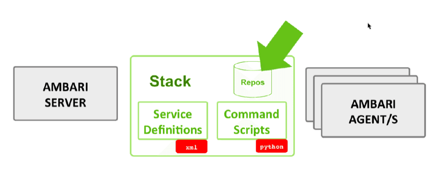
Special Bonus: Ambari Blueprints
This release also includes a technical preview of the Ambari Blueprints feature. With Ambari Blueprints, you can simplify the automation of cluster installs by defining the stack to use, the components layout and the configuration. With just a few API calls, you have a cluster up and running. This is particularly helpful for virtual and cloud environments where the Hadoop operator wants to create ad hoc discovery clusters or dev and test clusters, in an automated and consistent fashion.
The Apache Knox Gateway team is pleased to announce Knox’s first release as an Apache top-level project: Apache Knox Gateway 0.4.0. The team resolved approximately 100 JIRAs for this release and Knox Gateway is now better positioned to provide complete security for REST API access to a Hadoop cluster.
The new features in Knox Gateway 0.4.0 are the features that enterprise security officers expect in a gateway solution:
Perimeter security for a Hadoop cluster
Support for enterprise group lookup
Audit log of all gateway activity
Command line tooling for CMF provisioning
Protection for web application vulnerabilities
Pre-authentication via SSO token
And many more…
As a top-level project, Apache Knox Gateway is fully endorsed by the Apache Software Foundation, and this improves coordination between development of Knox and the other core Hadoop projects with which it interacts.
Here is more detail on some of the specific features in Knox 0.4.0.
Perimeter Security and Group Lookup Through Apache Shiro
We extended the Apache Shiro provider to pull group memberships from the LDAP directory. It also provides support for dynamic groups.
Group memberships, coupled with an ACL-based authorization provider, form a powerful solution for service-level authorization and perimeter security that can be elegantly integrated with the enterprise directory server.
Audit Log of all Gateway Activity
All interactions that pass through the gateway are recorded in an audit log. This includes the IP and principal of the caller and other relevant attributes of the user, service and resource.
Pluggability within the audit mechanism allows for the use of custom audit stores.
Command Line Tooling for Keys and Passwords
The KnoxCLI utility facilitates creation and management of security artifacts. This allows the user to:
Create the master secret,
Create and manage password/credential aliases and
Generate a self-signed certificate for use as the gateway identity certificate.
The KnoxCLI also provides commands for general gateway management services.
Protection for Web Application Vulnerabilities
This release introduces a Web App Security provider. Cross-site-scripting (CSRF) is the first web app vulnerability addressed for REST APIs, but the web app security provider is designed for extension to protect against other future vulnerabilities.
Pre-authentication Via an SSO Token
This feature allows the identity and groups from an external authentication to be propagated and trusted by the Knox Gateway server. It targets integrations with SSO solutions such as CA SiteMinder where HTTP Headers are used to assert the authenticated identity.
The Apache Knox Gateway community is already looking forward to the next release—to improve existing features and to add new protections for Hadoop clusters.
The Knox Gateway project is always looking for more security-savvy developers to contribute to our top-level project within the Apache Software Foundation and to develop the Hadoop ecosystem!
The first use of the term BoF session was used at the Digital Equipment Users’ Society (DECUS) conference in the 1960s. Its essence was to bring together like minds and thought leaders—just as birds of the feather flock together— to share and exchange computing ideas, in an informal yet spirited way. Since then, the organizers and sponsors of most computing conferences have been loyal to its essence and spirit.
For ideas and innovation happen in collaboration—not in isolation. Steven Johnson, in his talkWhere Good Ideas Come From, explains that most good ideas evolve over time. The best ones emerge from collaboration with other ideas. And nowhere is this true than in today’s open-source community, in the Apache Hadoop community—what the developers’ collaboration has achieved; what knowledge they have shared.
Knowledge, when acquired and shared, elevates societies. Plato is said to have remarked that knowledge is “the food of the soul.” And C.S. Lewis is said to have noted that education and literature “irrigates the deserts” of our lives. Well, I think that BoFs for developers and practitioners are the oasis through which we irrigate our dry deserts of computing knowledge. The BoFs are our modern equivalent of old coffee houses of creativity and activity, the equivalent of the Parisian cafes of conversation and collaboration, in our digital age of enlightenment
As you know, Hadoop Summit, San Jose is less than five weeks away. Hortonworks will sponsor several Birds of Feather (BoFs) sessions, hosted by Hortonworks’ architects, tech-leads, committers, and engineers. These sessions are not restricted to conference attendees; they’re open to everyone.
Here is the list where you can RSVP. Because they’re all being held at the same time, June 5 to you’ll have to pick and choose, but you can always wander among them.
Hadoop 2 and its YARN-based architecture has increased the interest in new engines to be run on Hadoop and one such workload is in-memory computing for machine learning and data science use cases. Apache Spark has emerged as an attractive option for this type of processing and today, we announce availability of our HDP 2.1 Tech Preview Component of Apache Spark. This is a key addition to the platform and brings another workload supported by YARN on HDP.
There has been a marked increase in interest among data scientists and enthusiasts for Apache Spark as they explore new ways to perform their very unique yet complex task in Hadoop. Our customers are investigating this technology as Spark allows key resources to effectively and simply implement iterative algorithms for advanced analytics such as clustering and classification of datasets. It provides three key value points to developers,
in-memory compute for iterative workloads,
a simplified programming model in Scala,
and machine learning libraries to simply programming.
The Hortonworks Commitment
Hortonworks’ tech preview of Apache Spark is part of a larger initiative that will bring the best of heterogeneous, tiered storage, and resource-based models of computing together with the broader Hadoop community starting at the core of HDFS and working outward from there.
Our focus remains on delivering a fast, safe, scalable, and manageable platform on a consistent footprint that includes HDFS, YARN, Tez, Ambari, Knox, and Falcon to name just a few of the critical components of enterprise Hadoop. We are working within this comprehensive set of components and hope to make Apache Spark “enterprise ready” so that our customers can confidently adopt it.
Availability
We have already completed baseline work to integrate Spark on YARN with HDP and want to make this available so that we work with customers to identify use cases which are best suited for this technology. Spark has the potential to meet the complex requirements of data science and machine learning use cases. We encourage you to download our Tech Preview today and engage us so we can build out this key technology together.
I’m a pretty heavy Unix user and I tend to prefer doing things the Unix Way™, which is to say, composing many small command line oriented utilities. With composability comes power and with specialization comes simplicity. Although, sometimes if two utilities are used all the time, sometimes it makes sense for either:
A utility that specializes in a very common use-case
One utility to provide basic functionality from another utility
For example, one thing that I find myself doing a lot of is searching a directory recursively for files that contain an expression:
Despite the fact that you can do this, specialized utilities, such as ack have come up to simplify this style of querying. Turns out, there’s also power in not having to consult the man pages all the time. Another example, is the interaction between uniq and sort. uniq presumes sorted data. Of course, you need not sort your data using the Unix utility sort, but often you find yourself with a flow such as this:
sort filename.dat | uniq > uniq.dat
This is so common that a -u flag was added to sort to support this flow, like so:
sort -u filename.dat > uniq.dat
Now, obviously, uniq has utilities beyond simply providing distinct output from a stream, such as providing counts for each distinct occurrence. Even so, it’s nice for the situation where you don’t need the full power of uniq for the minimal functionality of uniq to be a part of sort. These simple motivating examples got me thinking:
Are there opportunities for folding another command’s basic functionality into another command as a feature (or flag) as in sort and uniq?
Can we answer the above question in a principled, data-driven way?
This sounds like a great challenge and an even greater opportunity to try out a new (to me) analytics platform, Apache Spark. So, I’m going to take you through a little journey doing some simple analysis and illustrate the general steps. We’re going to cover
Data Gathering
Data Engineering
Data Analysis
Presentation of Results and Conclusions
We’ll close with my impressions of using Spark as an analytics platform. Hope you enjoy!
Data Gathering
Of course, to be data driven, a minimal requirement is to have some data. The good folks at CommandLineFu have a great service and an even better REST-ful API to use. For those of you who do not know, CommandLineFu is a repository of crowd-managed one-liners for common tasks. For instance, if you forget how to share ssh keys and you’re on a Mac that doesn’t have ssh-copy-id (like me), then you can find the appropriate one-liner. Using their REST-ful API, we can extract a nice sample of useful sets of commands to accomplish real tasks. Now, this data, unfortunately, leaves much to be desired for drawing robust conclusions:
Not a huge amount of data (only 4744 commands when I pulled the data)
Duplicity of commands aren’t captured (we’ve essentially just captured a unique list of commands).
Not captured from real-world usages, so it might be biased
Even so, perhaps we can see some high-level patterns emerge. At the very least, we’ll be able to try out a new analytics platform.
The Spark of Inspiration
Word Collocations as Inspiration
Word collocations (AKA Statistically Significant Phrases) are pairs (or tuples) of words that appear together more likely than random chance would imply. These could be things like proper names, multi-word colloquial phrases. Natural Language Processing has a number of techniques to generate and rank these collocations by “importance”:
Statistical Tests in Natural Language Processing for Fun and Profit
Statistical Test
Statistical significance tests tell us whether the probability that something occurs is not due to just random chance. Traditionally, when you are looking at these sorts of things, you encounter tests like the test, which can tell you give you a significance measure. In fact, G-tests, and their broader class of tests called maximum likelihood statistical tests, are a generalization of the test. In particular, the problem with the traditional test when used in the domain of natural language processing is well known and criticized. Consider the following quote from “Foundations of Statistical Natural Language Processing”:
Just as the application of the $t$ test is problematic becuase of the underlying normality assumption, so is the application of in cases where numbers in the $2$-by-$2$ table are small. Snedecore and Cochran(1989:127) advise against using if the total sample size is smaller than 20 or if it is between 20 adn 40 and the expected value in any of the cells is 5 or less.
As you can see, there are some issues with bigrams (in our case, pairs of commands) that are rare. Thankfully there is another approach that deals with the low-support situation.
G Statistical Test
The G statistical test is a maximum likelihood statistical significance test. In fact, it turns out, the test statistic is an approximation of the log-likelihood ratio used in the G statistical test. You can refer to Ted Dunning’s “Accurate Methods for Statistics of Surprise and Coincidence” for a spirited argument in favor of log-likelihood statistical tests as the basis of bigram collocation analysis.
Apache Spark: An Analytics Platform
As part of my career, I have specialized in Data Science on the Hadoop stack. Amp Labs at Berkeley have created some very interesting pieces of infrastructure with favorable performance characteristics and a functional flavor. Apache Spark is their offering at the computational layer. It’s a cache-aggressive data processing engine with first-class Scala, Java and Python API bindings. With Hadoop 2.x now supporting other communication models than MapReduce, Spark runs as a Yarn application; so if you have a modern Hadoop cluster, you can try this out yourself. Even if you don’t own a Hadoop cluster, you can pull down a VM that runs the full Hadoop stack here. (Disclosure: I work for Hortonworks; this is a VM with our distribution installed). As a fan of scala and data science, I would be lying if I said that I haven’t been looking forward to finding a project to try it out on, but I wanted something a bit more interesting than the canonical examples of wordcount or estimation. I think this just fits the bill!
The Analysis Process
Data Engineering
As part of any self-respecting data science project, a good portion of the challenge is in data engineering. The data engineering challenge here boil down to parsing the command line examples and extracting the pairs of commands that collocate. The general approach is:
Use Antlr, a parser generator which can take a grammar and give us back an abstract syntax tree, to parse the unix lines according to the grammar generously borrowed from the libbash project here.
Take those abstract syntax trees and extract out the pairs of commands.
If you’re interested, you can find the scala code to do this here.
Analysis: In the Weeds
The general methodology is:
Compute the raw frequency ranking of all of the pairs of commands that appear in our dataset
Compute the G test significance for all of the pairs of commands that appear in our dataset
Once we have these two rankings, we can eyeball the rankings and see how they differ and see if anything pops out.
Resilient Distributed Datasets: Our Workhorse
I want to briefly discuss a bit of technology that we will be using heavily in the ensuing analysis, the Resilient Distributed Dataset (aka RDD). Resilient Distributed Datasets:
Are Spark’s primary abstraction for a collection of items
Could back a HDFS file, a local Text file, or many other things.
Have many operations available on them that should be familiar to any functional programmer out there.
Are lazily operated on. In that, all transformations from above do not compute their results until their results are absolutely needed (such as when they’re persisted).
Take advantage of caching and, therefore, can cache a workingset into memory, thereby operating on it more quickly.
Generally when you want to get something done in Spark, you’re operating on an RDD.
Raw Frequency: The Baseline
Raw Frequency is really simple, so we’ll start with that. It fits our assumptions of how to rank collocations, so we’ll use it as the base-case to evaluate against. Let’s start with some useful typedefs
type Bigram = Tuple2[String, String]
type ScoredBigram = Tuple2[Bigram, Double]
type BigramCount = Tuple2[Bigram, Int]
Now, let’s define our function.
/**
   * Returns a RDD with a scored bigram based on frequency of consecutive commands.
   * @param commands an RDD containing Strings of commands
   * @return An RDD of ScoredBigram sorted by score
   */
  def rawFrequency(commands:RDD[String]) :RDD[ScoredBigram] =  {
Using the parser that we created during the Data Engineering portion of the project, we can extract the Bigrams excluding the automatic bookend command called “END” into an RDD called bigramsWithoutEnds.
val parser = new CLIParserDriver
    val commandsAsBigrams= commands.map( line => parser.toCommandBigrams(
        parser.getCommandTokens(parser.getSyntaxTree(line.toString))
                                                                        )
                                      )
    val bigramsWithoutEnds = commandsAsBigrams.flatMap(
            bigrams => bigrams.filter( (bigram:Bigram) => bigram._2 != "END")
                                                      )
Now we can compute the collocation counts by bigram by doing something very similar to word count using map and reduceByKey.
val bigramCounts = bigramsWithoutEnds.map( (bigram:Bigram) => (bigram, 1))
                                         .reduceByKey( (x:Int, y:Int) => x + y)
With those counts, we now need only the total of all bigrams and to divide each of the bigram counts by the total to get the raw frequency. We’ll further order by the score.
val totalNumBigrams = bigramsWithoutEnds.count()

    bigramCounts.map(
      (bigramCount:BigramCount) => ( 1.0*bigramCount._2/totalNumBigrams
                                   , bigramCount._1
                                   )
                    )
                .sortByKey(false) //sort the value (it's the first in the pair)
                .map( (x:Tuple2[Double, Bigram]) => (x._2, x._1)) //now invert the order of the pair
  }
Et voilà, we now have a RDD of Bigrams sorted by raw frequency.
The number of times and appear next to each other.
k12
The number of times appears without
k21
The number of times appears without
k22
The number of times neither or appear together.
Just as before with raw frequency, let’s start with some useful typedefs
type Bigram = Tuple2[String, String]
type ScoredBigram = Tuple2[Bigram, Double]
type BigramCount = Tuple2[Bigram, Int]
Again, just as before, let’s define our function:
/**
   * Returns a RDD with a scored bigram based on the G statistical test
   *  as popularized in Dunning, Ted (1993). Accurate Methods for the
   * Statistics of Surprise and Coincidence, Computational Linguistics,
   * Volume 19, issue 1 (March, 1993).
   *
   * @param commands an RDD containing Strings of commands
   * @return An RDD of ScoredBigram sorted by score
   */
  def g_2(commands:RDD[String]) :RDD[ScoredBigram] =  {
For the purposes of this analysis, it’s convenient to have an inner function which is useful for computing the G significance given some of the counts mentioned in the contingency table above.
/**
     * Returns the G score given command counts
     * @param p_xy The count of commands x and y consecutively
     * @param p_x The count of command x
     * @param p_y The count of command y
     * @param numCommands The total number of commands
     * @return The G score
     */
    def calculate(p_xy:Long, p_x:Long, p_y:Long, numCommands:Long) : Double = {
      val k11= p_xy // count of x and y together
      val k12= (p_x - p_xy) //count of x without y
      val k21= (p_y - p_xy) // count of y without x
      val k22= numCommands- (p_x + p_y - p_xy) //count of neither x nor y

      LogLikelihood.logLikelihoodRatio( k11.asInstanceOf[Long]
                                      , k12.asInstanceOf[Long]
                                      , k21.asInstanceOf[Long]
                                      , k22.asInstanceOf[Long]
                                      )
    }
So, again, the prelude is similar to the raw frequency case. Given a line, let’s compute the bigrams of commands.
val parser = new CLIParserDriver
    // Convert the commands to lists of command pairs
    val commandsAsBigrams= commands.map( line => parser.toCommandBigrams(
            parser.getCommandTokens(parser.getSyntaxTree(line.toString))
                                                                        )
                                       )
First, let’s get some statistics about individual commands. To do this, we need to count the individual commands (which are not the bookend “END” command that our CLIParserDriver puts in for us).
   /*
     * Count the individual commands
     */
    // Count the number of commands that are not END, a special end command
    // This is essentially command count
    val commandCounts = commandsAsBigrams.flatMap(
      (bigrams:List[Bigram] ) => bigrams.flatMap(
            (bigram:Bigram) => List(bigram._1, bigram._2)
                                                ).filter(x => x != "END")
                                                 )
                                         .map( (command:String) => (command, 1))
                                         .reduceByKey( (x:Int, y:Int) => x + y)
With Spark, we can pull down this RDD locally into memory into the Driver application. Since this scales only with the unique commands, it should be sensible to pull this data locally. We’re going to use these counts to create a map with which we can look up counts for a given command. Spark is going to ship that map to the cluster, so we can use it local to the transformations applied to the RDDs. This is a super useful bit of candy and unexpected for those of us coming from the traditional Hadoop stack (i.e. MapReduce and Pig development).
	// Collect the array of command to count pairs locally into an array
    val commandCountsArr = commandCounts.collect()
    // Create a Map from those pairs
    val commandCountsMap = Map(commandCountsArr:_*)
    //Count the values of command map to get the total number of commands
    val numCommands = commandCountsMap.foldLeft(0)( (acc, x) => acc + x._2)
Now that we’ve gotten some counts for individual commands, let’s do the same for pairs of collocated commands.
    /*
     * Count the bigrams
     */
    val bigramsWithoutEnds = commandsAsBigrams.flatMap(
        bigrams => bigrams.filter( (bigram:Bigram) => bigram._2 != "END")
                                                      )
    val bigramCounts = bigramsWithoutEnds.map( (bigram:Bigram) => (bigram, 1) )
                                         .reduceByKey( (x:Int, y:Int) => x + y)
    val totalNumBigrams = bigramsWithoutEnds.count()
Now that we have a RDD with the bigrams and their counts, bigramCounts, the map with the counts by individual command, commandCountsMap, we can compute our G statistical significance test for each pair of collocated commands.
/*
 * Score the bigrams using the individual command count map and the
 * bigram count RDD
 */
bigramCounts.map( (bigramCount:BigramCount) => (
  calculate( bigramCount._2 // The count of the pair of commands
           , commandCountsMap(bigramCount._1._1) //The count of the first command
           , commandCountsMap(bigramCount._1._2) //The count of the second command
           , numCommands // the total number of commands
           )
                                               , bigramCount._1 // the pair of commands
                                               )
                )
            .sortByKey(false) //sort the value (it's the first in the pair)
            .map( (x:Tuple2[Double, Bigram]) => (x._2, x._1)) //now invert the order
  }
Now, we have a RDD with the bigrams ranked by the G statistical significance test.
The Results
The result of this analysis is two rankings. One based on frequency and one based on G score. I’ve taken the top 10 results from each ranking and placed them in a table here along with their scores and relative rankings. Note that while the table is sorted by G score, the columns in the following table are sortable, so go explore. Also, for each score, the higher the score, the more important the pair of commands.
As you can see by sorting the absolute difference in rank ascending, there is much overlap between the two rankings
sort, uniq shows up second in the list for the G ranking, so at the very least this ranking can recover some of what our intuition indicates should be true.
The relative difference between all of the pairs of commands where grep is the second in the pair have G ranking much higher (e.g. sort, grep has a difference in ranking of 496). Intuitively, this feels right considering the situations where I use grep as a filtering utility after some processing (i.e. sort, awk, etc).
It is not proper, of course, to draw too many conclusions from an eyeball analysis as we are subject to humanity’s tendency to rationalize and find patterns to justify preconceived notions.
Conclusions
The secondary purpose for this project is to discuss Spark as a platform for Data science. I’ll break it down into pros and cons regarding Spark.
Fast, Featureful and Gets Things Done
Spark, contrary to traditional big data analytics platforms like Hadoop MapReduce, does not assume that caching is of no use. That being said, despite aggressive caching, they have worked hard to have graceful degradation when you cannot fit a working set into memory. This assumption is particularly true in data science, where you are refining a large dataset into a (possibly) much smaller dataset to operate on. The dominant pattern for modern big data analytics systems has always borrowed heavily from functional languages. Spark substantially reinforces this pattern. Not only did it choose a functional language, Scala, as a first-level programming language, but it borrowed most of your favorite higher-order functional primitives for collections or streams (e.g. foldl, foldr, flatMap, reduce, etc.).
Exists within a Popular Programming Environment
Existing within the JVM (for the Scala and Java API bindings) and Python ecosystem (for the Python bindings), comes with the ability to use libraries written for two of the most popular programming environments available today in a dead-simple way. Everything from Stanford CoreNLP to scikit-learn is available without any of the integration challenges that you see in the big data scripting languages (i.e. wrapping the calls in user defined functions).
Works on Hadoop
Spark did not try to bite off more than it could chew. The AmpLabs guys realized that resource allocation in distributed systems is hard and they chose, quite correctly, to separate the analytics framework from the resource allocation framework. Initially, and continuing to today, they have strong support for Apache Mesos. With the advent of Hadoop 2.0 resource management and scheduling have been abstracted into YARN. This means that Spark can now run on Hadoop, which comes with the distinct advantage that you can run Spark alongside the rest of the Hadoop ecosystem applications, such as Apache Hive, Apache Pig, etc. With Hadoop’s increased adoption into the data center as a batch analytics system for doing ETL, it substantially decreases the barrier to entry to have Spark available as it can use the same hardware. An open question, however, is just how good Spark is at multitenancy. If anyone has any examples of large Hadoop MapReduce-based workloads being run alongside Spark (as opposed to running in separate clusters), I’d love to hear impressions and challenges.
Oriented toward the coding data scientist
Almost all of the previous positive points tag my orientation as in the “comfortable with coding” type of data scientist. I have attempted to keep my foot in both worlds and that biases my perspective. Many people working and doing good analytics are daunted, to say the least, with a (new to them, most likely) language like Scala. That being said, I think that two points alleviate this criticism:
The SparkR package, intended to expose processing on RDDs and some of the RDD transformations to R.
These are attempts by the Spark community to reach out to the comfort-zone of the existing community of Data scientists by supporting some of their favorite tooling. I do not think that this will make someone who has had a career writing SAS comfortable in the system, unfortunately, but it does help.
Still Kind of Hard to Run
This is one of those things that gets fixed with maturity, but it’s a lot easier to run a Pig script, say, than a Spark app. For instance, running the canonical example from Spark, the estimator (from the docs):
# Submit Spark's ApplicationMaster to YARN's ResourceManager, and instruct Spark
# to run the SparkPi example
SPARK_JAR=./assembly/target/scala-2.10/spark-assembly-0.9.0-incubating-hadoop2.0.5-alpha.jar \
    ./bin/spark-class org.apache.spark.deploy.yarn.Client \
      --jar examples/target/scala-2.10/spark-examples-assembly-0.9.0-incubating.jar \
      --class org.apache.spark.examples.SparkPi \
      --args yarn-standalone \
      --num-workers 3 \
      --master-memory 4g \
      --worker-memory 2g \
      --worker-cores 1
A combination of sensible defaults, programmatic specifications which can be overridden from the command line and generally less magic would be very grateful here. Furthermore, after you do succeed in running this, you have to dig in logs to get what was printed out in stdout from the driver. Logs (again, straight out of the docs) like:
# Examine the output (replace $YARN_APP_ID in the following with the
# "application identifier" output by the previous command)
# (Note: YARN_APP_LOGS_DIR is usually /tmp/logs or $HADOOP_HOME/logs/userlogs
# depending on the Hadoop version.)
$ cat $YARN_APP_LOGS_DIR/$YARN_APP_ID/container*_000001/stdout
On the whole, I’m super interested in Spark. I like much about it and I’m especially interested in their ecosystem projects like MLLib. Chalk me up as a fan.
Source Code and Data
All of the code used to do this analysis is located here. I am not shipping the data, unfortunately, because I doubt that the commandlinefu guys would like me providing their data on my github repo. However, you can easily re-pull the data via their APIs.
This is the first post in our series on the motivations and architecture for improvements to the Apache Hadoop YARN’s Resource Manager Restart resiliency. Other in the series are:
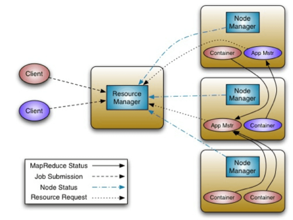
Resource Manager (RM) is the central authority of Apache Hadoop YARN for resource management and scheduling. It is responsible for allocation of resources to applications like Hadoop MapReduce jobs, Apache TEZ DAGs, and other applications running atop YARN. Therefore, though applications can continue to perform the scheduled work without interruption, the RM is a potential single point of failure in a YARN cluster, which is not acceptable in an enterprise production environment. To that end, the YARN community set out to plug this gap via various umbrella efforts.
The ultimate goal is to ensure that RM restart or fail-over is completely transparent to the end-users with zero or minimal impact to running applications. To this end, we split the effort into multiple phases
Phase I: Preserve application-queues: The focus of this phase is on enhancing the system so that ResourceManager can preserve application-queue state into a pluggable persistent state-store and reread that state automatically upon restart. Users should not be required to re-submit the applications. Existing applications in the queues should simply be re-triggered after RM restarts. This does not require YARN to save any running state in the ResourceManager – each application either simply runs from scratch after RM restarts or uses its own recovery mechanism to continue from where it left off.
YARN-128 is the umbrella Apache Hadoop YARN JIRA ticket that tracked this entire effort.
Phase II: Preserve work of running applications: Adding to the groundwork of phase I, this phase focuses on reconstructing the running state of the previous RM instance. By taking advantage of the recovered application-queues from phase I, combining that information with container-statuses from all the NodeManagers, and pulling together the allocation requests from the running ApplicationMasters in the cluster, RM restarts. Applications are not required to be restarted, as they will just re-sync with newly started RM. Thus no work will be lost due to a RM crash-reboot event.
This effort is still a TBD and is tracked in its entirety under the JIRA ticket YARN-556.
A related effort that takes advantage of the above phases of RM restart and enables a YARN cluster to be highly available is ‘RM-failover’:
RM failover: Tracked at YARN-149, this effort aims at supporting the ability to failover ResourceManager from one instance to another, potentially running on a different machine, for high availability. It involves leader election, transfer of resource-management authority to a newly elected leader, and client re-direction to the new leader.
In the next blog post, we will start with Phase I: application-queue-preserving restart of YARN ResourceManager. And the remaining phases are going to be covered as part of the subsequent posts.
This is the second in our series on the motivations and architecture for improvements to the Apache Hadoop YARN’s Resource Manager Restart resiliency. Other in the series are:
Introduction: Phase I – Preserve Application-queues
In the introductory blog, we previewed what RM Restart Phase I entails. In essence, we preserve the application-queue state into a persistent store and reread it upon RM restart, eliminating the need for users to resubmit their applications. Instead, the RM merely restarts them from scratch. This seamless restart of YARN apps in a production environment upon RM restart is imperative—it’s a necessity.
Rationale
As you may know, YARN in Hadoop 2 is an architectural upgrade of the MapReduce centric compute platform in Hadoop 1.x. The JobTracker of Hadoop 1.x is a single point of failure for the whole cluster. Any time the JobTracker is rebooted, it will essentially bring down the whole cluster. Even though clients persist their job specifications to HDFS, the states of their running jobs are completely lost.
A feature to address this limitation was implemented via HADOOP-3245 to let jobs survive JobTracker restarts, but it never attained production usage because of its instability. The complexity of that feature partly arose from the fact that JobTracker had to track and store too much information – both about the cluster state, as well as the scheduling status within each job.
The state of the art of JobTracker resiliency is thus shown below
JobTracker restart
The concern about separation of responsibilities is completely resolved with YARN’s distributed architecture ResourceManager. It is now only responsible for recovering application-queues and cluster status. Each application is responsible for persisting and recovering any application-level state. The separated concerns are obvious from the YARN’s control flow below:
YARN’s distributed architecture
Architecture
As stated before, RM-restart Phase I lets YARN continue functioning across RM restarts. RM may need to restart for various reasons – because of unexpected situations like bugs, hardware failures or because of deliberate and planned down-time during a cluster upgrade. RM restart now happens in a transparent manner. As such, users don’t need to explicitly monitor for such events and then manually resubmit jobs.
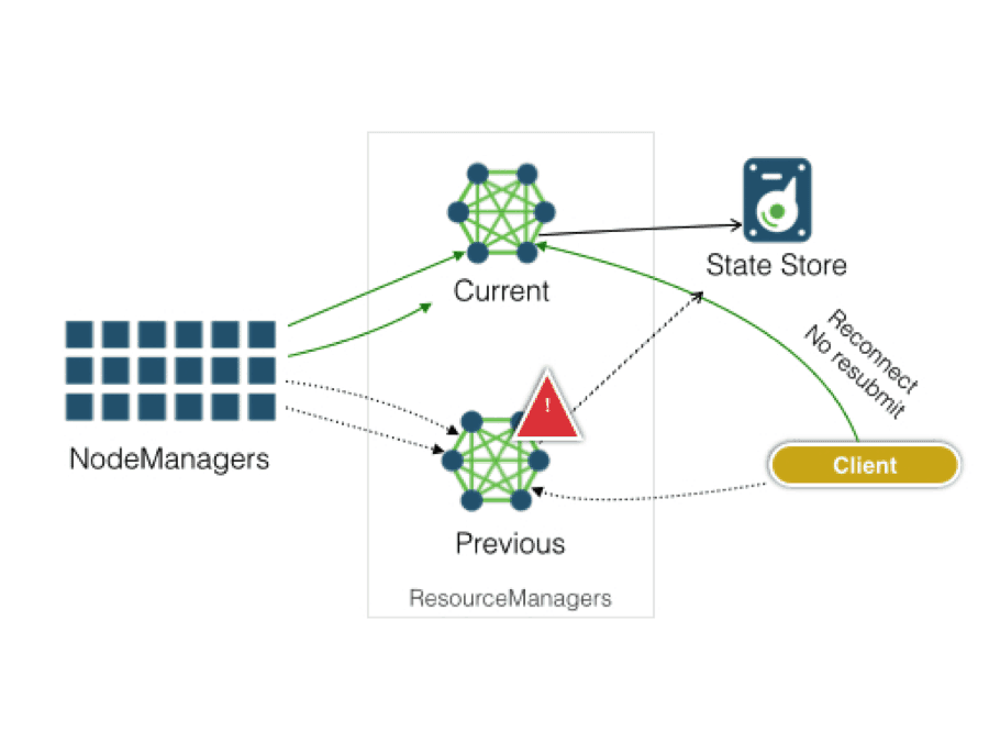
ResourceManager restart
There are a number of components and entities that facilitate a seamless RM resilience and restart.
ResourceManager state-store
In a persistent store called RMStateStore, the RM persists the application-queue state together with application-attempt state information. When RM restarts, it loads the state back into its memory. Additionally, RM also stores relevant security tokens or keys, so that the application’s previous security state is restored.
Today, the available state-store implementations are
ZKRMStateStore: A ZooKeeper-based state-store implementation
FileSystemRMStateStore: A state-store built on top of any FileSystems that are implemented using the Hadoop File-system interface, like for e.g. HDFS.
Below we describe what steps the RM follows to persist and restore an application state using a pluggable state-store. During the life-cycle of an application, RM does the following:
When an application is submitted or when an application-attempt is started, RM will first write the application/attempt state into the RMStateStore.
Similarly, when an application/attempt finishes, RM will record the final state of the application/attempt into the RMStateStore akin to write-ahead logging.
And then, specifically in RM restart Phase I, the RM does the following:
Any previously running applications are instructed to be shutdown or killed.
RM starts a new attempt of this application by taking the user’s original ApplicationSubmissionContext persisted on state-store and then runs a new instance of the ApplicationMaster.
Each restart, then, causes a new creation of an application-attempt. Therefore, AM-Max-Retry (the number of times RM can potentially relaunch the ApplicationMaster for any given application) count needs to be configured properly by users in their ApplicationSubmissionContext to allow the creation of a new attempt after RM restarts.
In the future, after RM restart Phase II, no new application-attempt will be created – the earlier running ApplicationMaster will just resync with the newly started RM and will resume its work.
When RM restarts, the clients are affected. In the following discourse, we attempt to explain how to handle them.
Clients
RMProxy – a library to connect to a ResourceManager
During a RM downtime, all the entities that were communicating with the RM – including ApplicationMaster, NodeManagers and the users’ clients – should be able to wait and retry until RM comes back up. We have written a library – RMProxy – that provides such an abstraction to wrap retry implementation. The retry behavior is configurable. But fundamentally, there is a wait interval between each retry, followed by more retries with a limit on the maximum wait-time. User applications can also take advantage of this proxy to communicate with RM instead of writing their own retry implementation.
The java client libraries YarnClient and AMRMClient already are modified to use the same proxy utility. So applications using these client-libraries get the above retry-functionality without any code changes!
NodeManager
When an RM is down, all the NodeManagers (NM) in the cluster wait till the RM comes back up. Upon RM’s restart, NMs are notified to reinitialize via a resync command from RM. In Phase I, NodeManagers handle this command by killing all the running containers (no need to preserve work) and re-register with RM. From the perspective of the newly started RM, these re-registered NMs will be treated just like newly joining NMs.
This is a chief reason why, in Phase I, running work of all the existing application is lost after RM restarts. In Phase II, NMs will instead not kill any running containers and simply report back the current container-statuses upon re-register with RM. This avoids the trouble of losing work, the overhead of launching new containers, reducing potential impact and observable losses in performance when you have a large cluster with many containers.
ApplicationMasters
Similarly to NMs, during the downtime of RM, ApplicationMasters (AM)—using the client-libraries or the RMProxy described above—will spin and retry until RM comes up. After RM is back to running as usual, all existing AMs will receive a resnyc command. The AMs today are expected to shutdown immediately when they receive a resync command.
Since an AM also runs on one of the containers managed by NM, it is also possible that, before an AM has a chance to receive the resync command, it is forcefully killed by NM’s kill signal while NM is resyncing with RM. In Phase I, users should be aware about this scenario that AM cannot totally rely on the resync command to perform RM restart handling logic. RM restart may cause the earlier running AM to be forcefully killed.
Configuration
To enable Phase 1 RM Restart, one can make the following config changes:
yarn.resourcemanager.recovery.enabled: The flag to enable/disable this feature. Defaults to false by default. If this configuration property is set to true, RM will enable the RM-restart functionality.
yarn.resourcemanager.store.class: Specifies the choice of the underlying state-store implementation for storing application and application-attempt state and other credential information to enable restart in a secure environment. The available state-store implementations are
org.apache.hadoop.yarn.server.resourcemanager.recovery.ZKRMStateStore—a ZooKeeper-based state-store implementation describe above and
org.apache.hadoop.yarn.server.resourcemanager.recovery.FileSystemRMStateStore – a state-store implementation persisting state on to any FileSystem like HDFS
yarn.resourcemanager.am.max-attempts: This configuration has an impact beyond the RM-restart functionality. It specifies the upper limit on number of application-attempts any application may have. Each application can specify its own individual limit on the number of application-attempts via the submission API ApplicationSubmissionContext.setMaxAppAttempts(int maxAppAttempts) to be a value greater than or equal to one, but the individual preference cannot be more than the global upper bound defined by this configuration property.
It has specific implications w.r.t RM-restart. As described earlier, in the Phase I implementation, every time RM restarts, it will kill the previously running application’s attempt (or more specifically the AM) and then will create a new attempt to re-kick the previously running application. As such, every RM restart will increase the attempt count for a running application by 1.
For MapReduce applications, users can set ‘mapreduce.am.max-attempts’ to be greater than 1 in their configuration.
Configurations for ZKRMStateStore only
yarn.resourcemanager.zk.state-store.address: Comma separated list of Host:Port pairs, each corresponding to a server in ZooKeeper cluster where RM state will be stored. This must be supplied when using org.apache.hadoop.yarn.server.resourcemanager.recovery.ZKRMStateStore as the value for yarn.resourcemanager.store.class. For example: 127.0.0.1:2181
yarn.resourcemanager.zk.state-store.parent-path: Full path of the ZooKeeper znode where RM state will be stored.
yarn.resourcemanager.zk.state-store.timeout.ms: Session timeout in milliseconds for ZooKeeper-client running inside the RM while connecting to ZooKeeper. This configuration is used by the ZooKeeper server to determine when a client session expires. Session expiration happens when the server does not hear from the client (i.e. no heartbeat) within the session timeout period specified by this configuration. Default value is 10 seconds.
yarn.resourcemanager.zk.state-store.num-retries: Number of times the ZooKeeper-client running inside the ZKRMStateStore tries to connect to ZooKeeper in case of connection timeouts. Default value is 500.
yarn.resourcemanager.zk-retry-interval-ms: The interval in milliseconds between each retry of the ZooKeeper client running inside the ZKRMStateStore when connecting to a ZooKeeper server. Default value is 2 seconds.
yarn.resourcemanager.zk.state-store.acl: ACL’s to be used for ZooKeeper znodes so that only the RM can read and write to the corresponding zk-node structure.
Configurations for FileSystemStateStore only
yarn.resourcemanager.fs.state-store.uri: URI pointing to the location of the FileSystem path where RM state should be stored. This must be set on the RM when FileSystemRMStateStore is configured to the state-store. An example of setting this for HDFS is hdfs://localhost:9000/rmstore which is writable and readable only by the RM.
If you point this to local file system like file:///tmp/yarn/rmstate, RM will choose the local file system as underlying persistent store. Note that, as discussed before, this will not be a useful setup for high-availability.
Conclusion and future-work
In this post, we have given an overview of the RM restart mechanism, how it preserves application queues as part of the Phase I implementation, how user-land applications or frameworks are impacted, and the related configurations. RM-restart is a critical feature that allows YARN to be able to continue functioning without being the choke point of failure.
The Hadoop community has also validated the integration of ecosystem projects beyond MapReduce, like Apache Hive, Apache Pig, Apache Oozie, etc. such that user queries, scripts or workflows continue to run without interruption in the event of a RM restart.
RM restart Phase I sets up the groundwork for RM restart Phase II (work-preserving restart) and RM High Availability, which we’ll explore in subsequent posts shortly.
Syncsort is a Hortonworks Certified Technology Partner and has over 40 years of experience helping organizations integrate big data…smarter. Keith Kohl, Director of Product Management, Syncsort, is our guest blogger. Below he talks about the importance of certification and how it benefits Syncsort’s customers and prospects interested in Hadoop.
Back in January, Syncsort announced our partnership with Hortonworks and the certification of DMX-h on HDP 2.0. I was also given the opportunity to write a guest BLOG on the Hortonworks site about HDP 2 and the GA of YARN (thanks Hortonworks!).
Syncsort integrates with Hadoop and HDP directly through YARN, making it easier for users to write and maintain MapReduce jobs graphically. If you want to see, there are a number of videos here.
The Hadoop ecosystem is moving quickly, and so are we here at Syncsort. With the new release of HDP 2.1, we are excited to announce the certification of DMX-h on HDP 2.1!
This means our mutual customers have the confidence that the products are integrated and work together out of the box. Additionally, through the YARN integration, the processing initiated by DMX-h within the HDP cluster will make better use of the resources and execute more efficiently. This certification reflects our ongoing commitment to continue to work with Hortonworks and contribute to Apache Hadoop projects for the benefit of the entire Big Data community. As I mentioned in my previous BLOG, ETL is a common use case for Hadoop, even if users don’t know they’re doing ETL—they could be calling it data refinement, data preparation, data management or something else. But ETL is the most common use case.
But the question is, weren’t these organizations doing ETL before? So, why are they switching to Hadoop? The answer is to move processing from platforms such as the data warehouse (doing ELT), to a cost effective environment such as Hadoop. I’ve heard this called data warehouse optimization or offload. This BLOG isn’t about offload, but you can read more about it here from us, and from Hortonworks. And you’re going to hear a lot more about offload from us…stay tuned!
Hortonworks did something pretty cool by providing users with a VM of a completely installed version of HDP called the Hortonnworks Sandbox. We took that Sandbox and gave users the ability to download DMX-h and install it on the Hortonworks Sandbox. We also include some sample job templates – like the use cases above – and sample data.
Rainstor is a Hortonworks Certified Technology Partner and provides an efficient database that reduces the cost, complexity and compliance risk of managing enterprise data. RainStor’s patented technology enables customers to cut infrastructure costs and scales anywhere; on-premise or in the cloud and natively on Hadoop. RainStor’s customers are 20 of the world’s largest communications providers and 10 of the biggest banks and financial services organizations.
Rainstor’s Mark Cusack, Chief Architect, writes about the benefits of certification on HDP 2.1.
RainStor and Hortonworks have been collaborating since January 2012, when RainStor joined the Hortonworks Technology Partner Program offering a Big Data Archive solution on Hadoop for analytics against historical data to meet both business and compliance demands.
This new certification goes much further, enabling Hortonworks’ customers to run RainStor natively on HDFS, while offering enterprise-grade security features – including data encryption and masking – integrated with a highly efficient data store that utilizes market-leading compression. RainStor was certified on a Kerberos-enabled HDP cluster running YARN, and was tested to ensure that RainStor’s compressed data files stored on HDFS remain fully accessible via Hive, Pig, and MapReduce, as well as RainStor’s own MPP SQL query engine, even when operating in a secure Hadoop environment.
HDP 2.1 provides an excellent compute and storage platform for Rainstor’s secure data archiving solution. With HDP, customers can scale out archives to address the need to store more records for longer, for both analytics and data governance purposes. We always ensure that RainStor is supported on the latest Hortonworks release, ensuring that our customers can take full advantage of new capabilities that become available as HDP moves forward.
RainStor provides a comprehensive portfolio of enterprise features running on HDP to ensure data privacy, protection against insider threats, and also adherence to strict data governance and a number of industry-specific compliance regulations. Active Archive use-cases include off-load from enterprise data warehouses for which RainStor has custom-built connectors, including bi-directional data movement between Teradata and RainStor. This environment generally comprises sensitive, critical data that has to be managed and secured to exacting standards, which RainStor delivers while leveraging the power and scale of Hadoop.
Last week Vinay Shukla and Kevin Minder hosted the first of our seven Discover HDP 2.1 webinars. Vinay and Kevin covered three important topics related to new Apache Hadoop security features in HDP 2.1:
REST API security with Apache Knox Gateway
HDFS security with Access Control Lists (ACLs)
SQL security and next-generation Hive authorization
We’re grateful to the many participants who joined and asked excellent questions. This is the complete list of questions that they asked, with the corresponding answers:
Question
Answer
Is Knox Gateway a single point of failure?
No. Traditional web load balancers can be used in front of Knox to provide HA and scalability.
My company is a Microsoft shop. Please provide information on how Hadoop can fit into my environment.
In Active Directory, can I set ACLs at the organization unit (OU) level?
The metadata associated with the HDFS ACLs is stored in the NameNode metadata name space. While the users and groups may come from AD, the actual ACLs are not managed there.
Is Knox limited to a certain set of Web APIs or is it extensible to handle more than Oozie, WebHCat, etc.?
It is extensible. Knox has a plug-in framework that supports “drop in” extensions.
Does Hive Authorization apply to Tez?
Yes. Hive Authorization does apply when Tez is being used.
Where does Apache Sentry fit in?
Apache Sentry is a good authorization solution. Unfortunately, it does not provide a SQL standard-based authorization. With Sentry, the authorization policy is not stored in the same place where the table is, so if you drop a table, you’ll have to keep the policy in sync.
I see there are encryption features coming in Phase 3. When will Phase 3 be complete?
Phase 3 will be delivered over the next few releases of HDP. Exact dates are still TBD. Watch our Security for Enterprise Hadooplabs page for updates on the roadmap.
There is no doubt that Hadoop has proven value for many companies via more efficient use of resources or through new business value derived from new sets of data. However, the limited availability of trained personnel that have the necessary skills to develop and integrate with Hadoop has proven difficult for many organizations to overcome.
Please join Talend and Hortonworks on this webinar where we present an end-to-end use case across data load, processing and delivery of results for analysis of machine/sensor data without writing a line of code. Learn how Talend Big Data can shortcut your path to Hadoop expertise by:
Simplify Hadoop through the drag-n-drop designer for MapReduce
Rapidly iterate and develop with debugging and deployment tools
On May 15, Owen O’Malley and Carter Shanklin hosted the second of our seven Discover HDP 2.1 webinars. Owen and Carter discussed the Stinger Initiative and the improvements to Apache Hive that are included in HDP 2.1:
Faster queries with Hive on Tez, vectorized query execution and a cost-based optimizer
We’re grateful to the many participants who joined this webinar and asked excellent questions. Here’s the complete Q & A from the webinar:
Question
Answer
Are you using the Tez engine for processing these queries?
Yes. We used Tez for all queries in the demo. Notice that the output of the query is different for Tez than it would be for MapReduce.
Does Tez leverage in-memory processing?
Yes. There are various ways in which we take advantage of memory. We automatically figure out which tables to bring into memory and then stream the large table through that. The older versions of Hive could not do that.
Are there any plans to integrate ORC with other tools like Crunch, Cascading, Spark, Giraph?
Yes. We’ve got plans on our roadmap to have native support for Cascading, Crunch, and other services. We’ve already introduced native ORCFile support for Pig. We still have some additional work to completely decouple that from the Hive engine so that it’s very easy to use outside of Hive.
Does Hive use only one reducer?
No. It depends on what you’re doing. Hive will automatically decide how many reducers it thinks it needs. There are certain operations (e.g. order by) where you have to use one reducer only, but Hive will automatically ascertain how many reducers it will need.
Are ORC stats used to optimize the number of map tasks? For example, if I have very wide table, but I want to read only two columns, will Tez/Hive be able to notice this fact and start fewer tasks than needed for a full table scan?
We are improving the statistics gathering for Hive 0.14. The cost-based optimizer is a main thrust for Hive 0.14, and it will use the stats to scale up or scale down the job appropriately.
For this demo, are you using this Ambari 1.5.1?
Yes. We showed Ambari 1.5.1.
When should you not use Tez with Hive?
Tez does not support a couple of Hive features yet such as SMB Join, SELECT TRANSFORM and Indexes. So for now, you should still run those queries on MapReduce.
The reverse of that question is, “When should I use Hive on Tez?” If you need interactive query, you need to use Hive on Tez.
The long-term direction of the roadmap is to completely replace MapReduce with Tez.
Can you compare the performance of Hive on Tez with Impala?
Absolutely. We see people doing that every day. If you compare, make sure that you see how the systems perform at scale and under a variety of workloads. Don’t make a decision using 5 GB of data.
Make sure to use a large amount of data and use the SQL semantics that you need for deep processing of the data. Hive has many more SQL features than you’ll get for other SQL tools for Hadoop.
What is the maximum number of joins that can perform a query? Can we use outer – left – right – inner joins?
One query we regularly run has a 9-way join with a mixture of inner and left outer joins. There’s no hard-coded limit to the number of joins in one query. Hive on MR and Hive on Tez support all the same join types.
According to New York Observer, there were couple of major social reasons that spurred the genesis and growth of Meetup.com. First, it was Robert Putman’s book Bowling Alone, in which he talks about the collapse of communities in America. And the second was an event that not only changed the world but changed New York: it was the aftermath of September 11, where strangers cared about greeting, meeting, and talking. They yearned for a return of a community, with common interests, said Mr. Meeker, the founder of Meetup.com. Since 2001, the meetups around the world have flourished: To date, there are over 142,319 meetups, in 196 countries, with close to 16 million members.
In that global spirit of Meetup.com—to bring together people with common interests and ideas and to bring together a community of practitioners and developers—we have a menagerie of meetups covering all things Hadoop, all with fantastic speakers—from Big Data Science to Big Data-Driven Applications, from SQL on Hadoop to YARN Deep Dive.
Everyone can attend, including the reception for greeting, meeting, and networking. As you know, Hadoop Summit in San Jose is approaching fast. Below are all the meetups open for RSVP.
Monday, June 2nd
Cocktail Reception at the San Jose Hilton Hotel, Almaden Room, from 5:00 pm-6:30 pm, followed by the following Meetups, from 6:30 pm-10:00 pm, at their respective locations.
On Wednesday May 21, Himanshu Bari (Hortonworks’ senior product manager), Venkatesh Seetharam (committer to Apache Falcon), and Justin Sears ( Hortonworks’ Product Marketing Manager), hosted the third of our seven Discover HDP 2.1 webinars. Himanshu and Venkatesh discussed data governance in Hadoop through Apache Falcon that is included in HDP 2.1. As most of you know, ingesting data into Hadoop is one thing; having data governed, by dictating and defining data-pipeline policies, is another thing—a necessity in the enterprise.
In this informative discourse, the speakers explored and discussed:
Why you need Apache Falcon
What are some key new Falcon features
Showed a Demo highlighting how to:
define data pipelines with replication
declare policies for retention and late data arrival
We recently shipped HDP 2.1, and Apache Falcon is part of that GA release.
Can you use Falcon UI to manage Falcon entities and pipelines?
Today, the Falcon UI is read-only. You cannot edit it. But it’s something we are working on, and it’ll be available soon.
Amabari is not supported on Ubuntu yet (AFAIK), what about Falcon?
You are correct, Ambari support on Ubuntu is in the works, but Falcon already comes with debs and you could install it outside of Ambari. Note that HDP is supported on Ubuntu today; however, Ambari will have Ubuntu support in the near future.
How do I manage a Falcon server without Ambari today? Should I use Falcon UI?
You cannot manage Falcon nor monitor Falcon today in Ambari on Ubuntu. You have a minimal dashboard for Falcon to monitor the jobs. But eventually, you will soon be able to create and manage the pipelines in the UI
Do we have a UI for all this configuration?
We are working on the UI to enhance configuration management.
For this demo, are you using Ambari 1.5.1?
Yes. We showed Ambari 1.5.1.
Does Apache Falcon run on earlier versions of HDP too? Like, HDP 1.3, by any chance?
And if you have any further questions pertaining to Apache Falcon—documentation, code examples, tutorials—please post them on the Community forums under Falcon.
The Apache Ambari community is happy to announce last week’s release of Apache Ambari 1.6.0, which includes exciting new capabilities and resolves 288 JIRA issues.
Many thanks to all of the contributors in the Apache Ambari community for the collaboration to deliver 1.6.0, especially with Blueprints, a crucial feature that enables rapid instantiation and replication of clusters.
Each release of Ambari makes substantial strides in providing functionality to simplify the lives of system administrators and dev-ops engineers to deploy, manage, and monitor large Hadoop clusters, including those running on Hortonworks Data Platform 2.1 (HDP).
Key features in 1.6.0 that empower administrators and extend Ambari’s core operational functionality include:
Ambari Blueprints
Ambari Stacks and Stacks REST API
PostgreSQL support for Ambari DB, Hive Metastore and Oozie
Feature Details
Ambari Blueprints
System administrators and dev-ops engineers requested blueprints to speed the process of provisioning a cluster. Blueprints can be re-used, which facilitates easy configuration and automation for each successive cluster.
As the name suggests, Ambari Blueprints describe the architectural footprint of a stack and how individual components are laid out on each node. A stack definition coupled with a component layout comprises an Ambari Blueprint.
In short, an Ambari Blueprint allows an operator to instantiate a Hadoop cluster quickly—and reuse the blueprint to replicate cluster instances elsewhere, for example, as development and test clusters, staging clusters, performance testing clusters, or co-located clusters.
Ambari Stacks and Stacks REST API
Stacks enable Ambari operators to customize Ambari through a configuration-driven extensibility model. An Ambari Stack defines services, components, configurations, and repositories for a given stack, and wraps them in a consistent operational lifecycle with customizable command scripts. This makes plugging in and extending Ambari possible with minimal coding via a Stack Definition. Ambari 1.6.0 exposes these Stack definitions via the Stacks REST API.
PostgreSQL Support
Ambari now extends database support for Ambari DB, Hive and Oozie to include PostgreSQL. This means that Ambari now provides support for the key databases used in enterprises today: PostgreSQL, MySQL and Oracle. The PostgreSQL configuration choice is reflected in this database support matrix.
What to do with all that memory in a Hadoop cluster? The question is frequently heard. Should we load all of our data into memory to process it? Unfortunately the answer isn’t quite that simple.
The goal should be to put memory into its right place in the storage hierarchy, alongside disk and solid-state drives (SSD). Data should reside in the right place for how it is being used, and should be organized appropriately for where it resides. These capabilities should be available to all applications that use Hadoop, and should not require a lot of configuration to make them work efficiently.
These are ambitious goals. In this article, I propose a solution, a new kind of data set called the Discardable, In-Memory, Materialized Query (DIMMQ) and its three key underlying concepts:
Materialized queries,
Memory-resident data, and
Discardable data.
I shall explain how these concepts build on existing Hadoop facilities, are important and useful individually, combine to exploit memory, and balance the needs of various applications. Taken together they radically alter the performance characteristics and manageability of a Hadoop cluster.
Implementing DIMMQs will require changes at the query level (optimization queries in SQL and other languages such as Pig and Cascading) and also at the storage level. In an companion blog, Sanjay Radia proposes a Discardable Distributed Memory(DDM) for HDFS, a mechanism intended to support DIMMQs.
By the way, don’t ask me how to pronounce DIMMQ! I won’t mind at all if the name goes away, and the concepts surface in mundane-sounding features like “CREATE MATERIALIZED VIEW”. The important part is the concepts, and how they fit together.
Before I describe the concepts and vision in detail, let’s look at the trends in hardware, workloads, and data lifecycles that are driving this.
Hardware trends
The trend in hardware is towards heterogenous storage, a balance of memory, SSD and disk.
Table 1 shows the hardware configuration of a server in a Hadoop cluster, now versus 5 years ago. (The configurations are anecdotal, but fairly typical; both servers cost approximately $5,000.)
The data shows a gradual move towards memory, but there are no signs that disk is going away. We are not moving to an “all-memory architecture”; if anything, with the arrival of SSD, the storage hierarchy is becoming more complex, and memory will be an important part of it.
Table 1: Hardware Trends
Year
Cores
Memory
SSD
Disk
Disk : memory ratio
2009
4-8
8 GB
None
4 x 1 TB
512:1
2014
24
128 GB
1 TB
12 x 4 TB
384:1
Workloads and data lifecycles
Traditionally Hadoop has been used for storing data, and for batch analytics to retrieve that data. But increasingly it is used for other workloads, such as interactive analytics, machine learning, and streaming. There is a continuum of desired latency, from hours to milliseconds.
If we look at the life cycle of a particular data item, we also see a continuum. Some data might live on disk for years until it is structured and analyzed; other data might need to be acted upon within seconds or even milliseconds. An analyst or machine-learning algorithm might start using a subset of that data for analysis, creating derived or cleaned data sets and combining with the original data.
In general, fresh data is more likely to be read and modified, and activity drops off exponentially over time. But a subset of historic data might become “hot” for a few minutes or days, before becoming latent again. Clearly we would like the hot data to be in memory, but without rewriting our application or excessive tuning.
A pool of resources
Hadoop’s strength is that it brings all of the data in a cluster of computers, and the resources to process it, into a pool. This yields economies of scale. If you and I store our data in the same cluster, and I am not accessing my data right now, you can use my slice of the cluster’s resources to process your data faster.
Along with CPU cycles and network and disk I/O, memory is one of those key resources. Memory can help deliver high performance on a wide variety of workloads, but to maximize the use of memory, we need to add it to the pool, and make it easy for tasks to share memory according to their need, and make it easy for data to migrate between memory and other storage media.
What is the right model for memory?
Data management systems traditionally use memory in two ways. First, a buffer-cache stores copies of disk blocks in memory so that if a block is used multiple times, it only needs to be read from disk once. Second, query-processing algorithms need operating memory. Most algorithms use modest amounts of memory, but algorithms that work on collections (sort, aggregation and join) require large amounts of memory for short periods in order to operate efficiently.
For many analytic workloads, a buffer cache is not an effective use of memory. Consider a table that is 10x larger than available memory. A query that sums every row in the table will read every block once. If you run the query again, no matter how smartly you cache blocks, you will need at least 90% of the blocks again. If all the data is accessed uniformly, random reads will also experience a cache hit-rate of only 10%.
A Discardable, In-Memory, Materialized Query (DIMMQ) allows a new mode of memory use.
A materialized query is a dataset whose contents are guaranteed to be the same as executing a particular query, called the defining query of the DIMMQ. Therefore any query that could be satisfied using that defining query can also be satisfied using the DIMMQ, possibly a lot faster.
Discardable means that the system can throw it away.
In-memory means that the contents of the dataset reside in the memory of one or more nodes in the Hadoop cluster.
Let’s look at the advantages DIMMQs bring.
The defining query provides a link between the DIMMQ and the underlying dataset that the system can understand. The system can rewrite queries to use the DIMMQ without the application explicitly referencing it.
Because the rewrite to use the DIMMQ is performed automatically by the system, not by the application, it makes it OK for the system to discard the DIMMQ.
Because DIMMQs are discardable, we don’t have to worry about creating too many of them. Various sources (users, applications, agents) continually suggest DIMMQs, and the system continually throws out the ones that are not pulling their weight. This dynamic process optimizes the system without requiring any part of it be omniscient or prescient.
Building DIMMQs
How to introduce these capabilities to Hadoop? The architectural approach is compelling because we can build the core concepts separately, and we can evolve existing Hadoop systems such as HDFS, HCatalog, Tez and Hive.
It is tempting to make HDFS intelligent enough to recognize patterns and to rebuild DIMMQs that it had previously discarded. But that would introduce too much coupling into the system — in particular, HDFS would become dependent on high level concepts like HCatalog and a query-optimizer.
Instead, the design is elegantly stupid. The low-level system, HDFS, stores and retrieves DIMMQ data sets, and is allowed to discard them. A query optimizer in the high-level system (such as Hive or Pig) processes incoming queries and rewrites them in terms of DIMMQs. A user or agent builds DIMMQs speculatively, not directly controlling whether they are discarded, but knowing that HDFS will discard them if they do not pull their weight.
The core concepts — materialized queries, discardable data, and in-memory data — are loosely coupled and can be developed and improved independently of each other.
Work is already underway in Optiq to support materialized views, or more specifically, materialized query recognition. Optiq is a query-optimization engine and is already used in Hive as part of the CBO project.
Support for in-memory data is being planned in JIRA HDFS-5851.
Discardable data is an extension to HDFS’s long-standing support for replication (multiple copies of data on disk) and caching (additional copies in memory).
Sanjay Radia describes HDFS Discardable Distributed Memory (DDM), a mechanism that combines in-memory data, replication and caching, in a an upcoming blog post.
The Stinger vectorization initiative makes memory access more efficient by organizing data in column-oriented ranges. This reduces memory usage and makes for more efficient use of processor cache.
Other components, such as agents to gather statistics, recommend, build and maintain DIMMQs, can be built around the system without affecting its core parts.
Queries, materialized views, and caching
When a data management system such as Hadoop loads a data set into memory for more efficient processing, it is doing something that databases have always done: create a copy of the data, organized in a way that is more efficient for the task at hand, and that can be added or removed without the application’s knowledge.
B-tree indexes are perhaps the most familiar example, but there are also hash clusters, aggregate tables, remote snapshots, projections. Sometimes the copy is in a different medium (memory versus disk); sometimes the copy is organized differently (a b-tree index is sorted on a particular key, whereas the underlying table is not sorted); and sometimes the copy is a derived data set, for example a subset over a given time range or a summary.
Why create these copies? If the system knows about the copies of a data set, then it can use a copy to answer a query rather than the original data set. Queries answered that way can be several orders of magnitude faster, especially when the copy is in-memory and/or significantly smaller than the original.
The major databases (Oracle, IBM DB2, Teradata, Microsoft SQL Server) all have a feature called (with a few syntactic variations) materialized views. A materialized view consists of a SQL query and a table that contains the result of that query. For instance, here is how a materialized view might be defined in Hive:
CREATE MATERIALIZED VIEW emp_summary AS
 SELECT deptno, gender, COUNT(*) AS c, SUM(salary) AS s
 FROM emp>
 GROUP BY deptno, gender;
A materialized view is a table, so you can query it directly:
SELECT deptno FROM emp_summary
 WHERE gender = ‘M’ AND c > 20;
More importantly, it can be used to answer queries on other tables. Given a query on the emp table,
 SELECT deptno, AVG(salary) AS average_sal
 FROM emp WHERE gender = ‘F'
 GROUP BY deptno;
The planner can rewrite to use the emp_summary table, as follows:
SELECT deptno, s / c AS average_sal
 FROM emp_summary WHERE gender = ‘F’
 GROUP BY deptno;
emp_summary has done much of the work required to answer the query, so the results come back faster. It is also significantly smaller, so the memory budget required to keep it in cache is smaller.
From materialized views to DIMMQs
DIMMQs are an extension to materialized views.
First, we need to make the materialized query accessible to all applications written in all languages, so we convert it to Optiq’s language-independent relational algebra and store its definition in HCatalog.
Next, we tell HDFS that the materialized query (a) should be kept in memory, (b) can be discarded. This can be accomplished using hints on the file that underlies the table.
Other possible hints might tell HDFS whether to consider copying a DIMMQ to disk before discarding it, and estimates of the number of reads over the next hour, day, and month, to predict the DIMMQ’s usefulness. A materialized view that is likely to be used very soon is a good candidate to be stored in memory; if after a few hours the reads decline to a trickle, it might be worth paging it to disk rather than discarding if it is much smaller than the original data.
Lastly, we need a mechanism to suggest, create and populate DIMMQs. Here are a few:
Materialized views can be created explicitly, using CREATE MATERIALIZED VIEW syntax.
Perform incremental updates to materialized views using Apache Falcon
The system caches query results (or intermediate results) as DIMMQs.
An automatic recommender (based on ideas such as Data Cubes ) could suggest and build DIMMQs.
Respectively, these provide control to an administrator, the ability to adapt to new workloads, and optimization of the system based on past activity. We would recommend that systems use a blend of all three.
Variations on a theme
There are many ways that core concepts behind DIMMQs can be used and extended. Here are a few initial ideas, and we trust that the Hadoop community will find many more.
Materialized queries don’t have to be in-memory. A materialized query stored on disk would still be useful if, for example, the source dataset rarely changes and the materialized query is much smaller.
Materialized queries don’t have to be discardable, especially if they are on disk, where space is not generally a scarce resource. They will typically be deleted if they are out of sync with their source data.
Materialized queries don’t have to be specified in SQL. Other languages, such as Pig, Cascading, and Scalding, and in fact any application that uses Tez, should be able to use this facility.
Materialized query recognition is just part of the problem. It would be useful if Hadoop helped maintain the materialized query as the underlying data changes, or if you could tell Hadoop that the materialized query was no longer valid. We can build on ACID transactions work already started.
Materialized queries allow a wide variety of derived data structures to be described: summary tables, b-tree indexes (basically sorted projections), partitioned tables and remote snapshots are a few examples. Using the materialized query mechanism, applications can design their own derived data structures and have them automatically recognized by the system.
In-memory tables don’t have to be materialized queries. There are other good reasons to support in-memory tables. In a streaming scenario, for instance, you would write to an in-memory table first, and periodically flush to disk.
Materialized queries can help with data aging. As data gets older, it is accessed less frequently, and so you might wish to store it in slower and cheaper storage, at a lower replication level, or with less coverage by aggregate tables.
Conclusion
Discardable In-memory Materialized Query (DIMMQ) data sets express how our applications use data in a way that allows Hadoop to automatically optimize and adapt how that data is stored, in particular, storing copies of that data in memory.
DIMMQs are superior to alternative uses of memory. Unlike low-level buffer cache, DIMMQ caches high-level results, which can be much smaller and are closer to the required result. And unlike non-declarative materializations like Spark RDDs, an application can use a DIMMQ even if it doesn’t know that it exists.
DIMMQ is built from three concepts: materialized query recognition, in-memory data sets, and discardable data sets. Together, they allow applications to seamlessly use heterogeneous storage — disk, SSD and memory — and quickly adapt to changing patterns of data use. And they provide a new level of data independence that will allow the Hadoop ecosystem to develop novel data organizations.
Materializations combined with HDFS Discardable Distributed Memory (DDM) storage are a major advance in Hadoop architecture that build on Hadoop’s existing strengths and make Hadoop as the place to store and process all of your enterprise’s data.
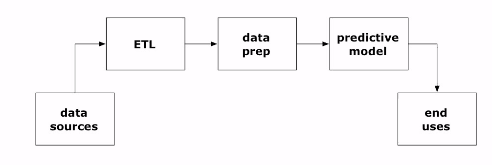
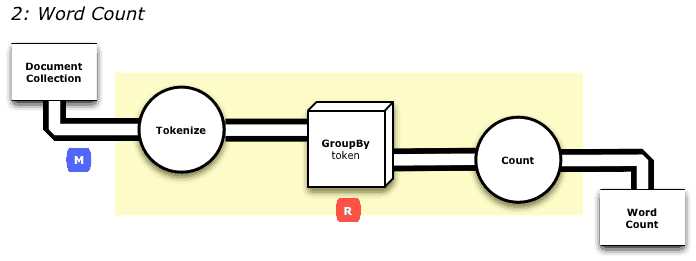
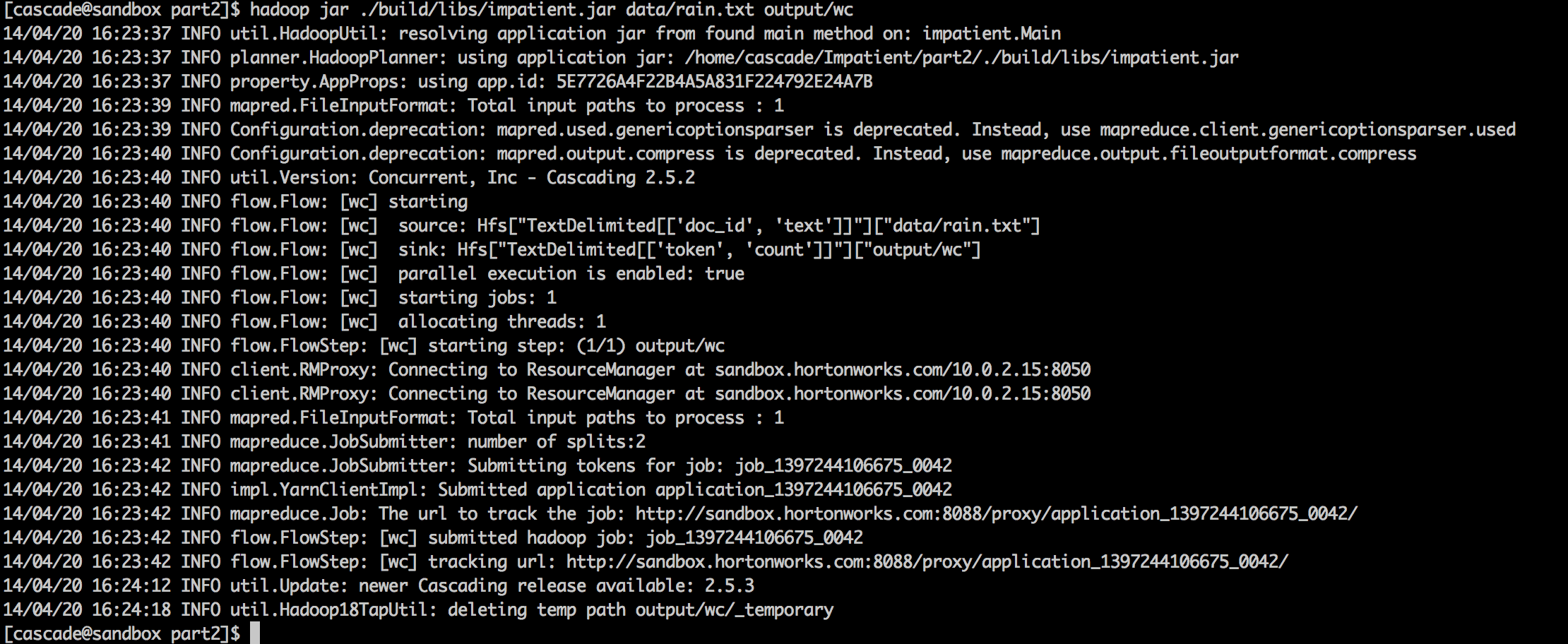

 Yesterday the
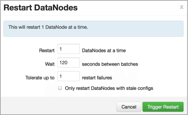
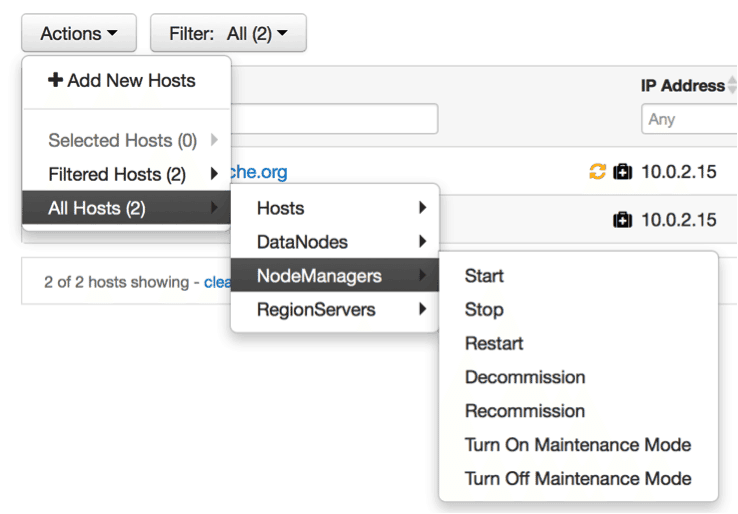
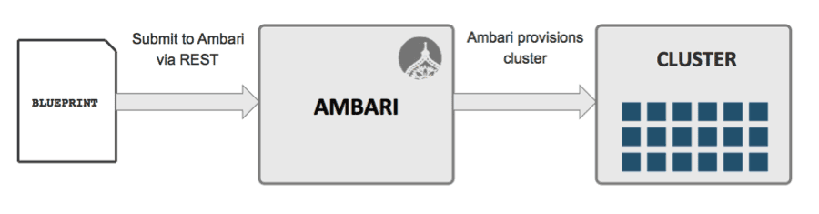
 The
The  Statistical Test
 estimation. I think this just fits the bill!
 and
and  and use
 Fast, Featureful and Gets Things Done
 Oriented toward the coding data scientist